On-Chain Data as Trading Signals: Funding Rates, OI, and Liquidation Zones
How to use on-chain perpetual futures data — funding rates, open interest, and liquidation heatmaps — as quantitative trading signals. Python implementations and backtest results on crypto markets.
The Data Nobody Uses Properly
Crypto perpetual futures generate a stream of on-chain data that has no equivalent in traditional markets. Funding rates, open interest, liquidation levels — these are direct windows into trader positioning that equity and forex markets simply don’t provide.
Most traders glance at funding rates on a dashboard and move on. We built quantitative signals from them.
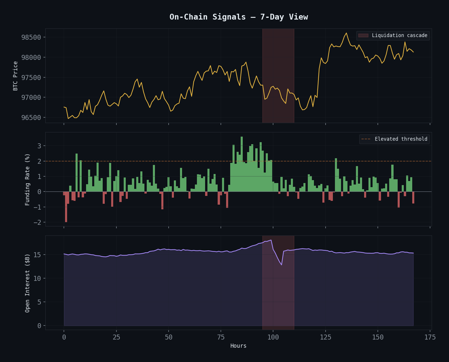 Real-time monitoring: price action, funding rate bars (green=positive, red=negative), and open interest accumulation. The cascade zone (red) shows where OI unwinds violently.
Signal 1: Funding Rate Extremes
Perpetual futures use funding rates to keep the perp price anchored to spot. When longs pay shorts (positive funding), the market is net long. When shorts pay longs (negative funding), the market is net short.
The signal: extreme funding rates tend to revert. When everyone is positioned the same way, the market tends to move against the crowd.
import numpy as np
import pandas as pd

def funding_rate_signal(
    funding_history: pd.DataFrame,
    lookback_hours: int = 168,  # 7 days
    z_threshold: float = 2.0,
) -> pd.DataFrame:
    """
    Generate mean-reversion signals from funding rate extremes.

    funding_history: DataFrame with 'timestamp' and 'funding_rate' columns
                     (typically 8-hour intervals on most exchanges)
    """
    df = funding_history.copy()

    # Cumulative funding over lookback (total cost of holding)
    intervals_per_day = 3  # 8-hour funding intervals
    lookback_intervals = (lookback_hours // 8)

    df['cum_funding'] = df['funding_rate'].rolling(lookback_intervals).sum()

    # Z-score of cumulative funding
    df['funding_mean'] = df['cum_funding'].rolling(lookback_intervals * 4).mean()
    df['funding_std'] = df['cum_funding'].rolling(lookback_intervals * 4).std()
    df['funding_z'] = (df['cum_funding'] - df['funding_mean']) / df['funding_std']

    # Signals: fade extreme positioning
    df['signal'] = 0
    df.loc[df['funding_z'] > z_threshold, 'signal'] = -1     # Too many longs -> short
    df.loc[df['funding_z'] < -z_threshold, 'signal'] = 1     # Too many shorts -> long

    # Annualized funding cost for context
    df['annualized_funding'] = df['cum_funding'] / lookback_intervals * intervals_per_day * 365

    return df
Backtest Results: BTC Funding Rate Reversion
| Metric | Value |
|---|---|
| Period | 2022–2025 |
| Trades | 89 |
| Win Rate | 58.4% |
| Profit Factor | 1.52 |
| Avg. Hold Time | 3.2 days |
| Max Drawdown | -11.3% |
The win rate and profit factor are strong, but the trade count is low. We need more data to be confident. This signal fires infrequently — about twice per month — because truly extreme funding is rare.
Important caveat: Funding rate extremes during genuine trend changes (like the 2022 LUNA collapse) can persist longer than you can stay solvent. We use a fixed stop-loss at 3 ATR to cap risk.
Signal 2: Open Interest Divergence
Open interest (OI) measures the total number of outstanding perpetual futures contracts. Rising OI means new money is entering the market. Falling OI means positions are being closed.
The most useful signal isn’t OI itself but OI-price divergence: when OI rises while price falls (or vice versa).
def oi_divergence_signal(
    df: pd.DataFrame,
    oi_lookback: int = 24,     # hours
    price_lookback: int = 24,
    divergence_threshold: float = 0.5,  # ATR units
) -> pd.DataFrame:
    """
    Detect divergence between open interest and price movement.

    Bearish divergence: OI rising + price rising = new shorts entering at higher prices
                        (they'll need to cover, adding to upside... or they're right)
    Bullish divergence: OI rising + price falling = new longs entering at lower prices
                        (they'll capitulate adding to downside... or they're right)

    The key: combine with funding rate direction to disambiguate.
    """
    df = df.copy()

    # OI change (percentage)
    df['oi_change'] = df['open_interest'].pct_change(oi_lookback) * 100

    # Price change
    df['price_change'] = df['close'].pct_change(price_lookback) * 100

    # Divergence score: positive means OI and price moving opposite
    df['divergence'] = df['oi_change'] * -np.sign(df['price_change'])

    # Normalize by ATR for cross-asset comparability
    atr = df['close'].pct_change().rolling(24 * 14).std() * np.sqrt(24) * 100
    df['divergence_norm'] = df['divergence'] / atr

    # Combine with funding direction
    if 'funding_rate' in df.columns:
        # OI up + price down + positive funding = longs trapped, bearish
        df['trapped_longs'] = (
            (df['oi_change'] > 5) &
            (df['price_change'] < -1) &
            (df['funding_rate'] > 0.01)
        )
        # OI up + price up + negative funding = shorts trapped, bullish
        df['trapped_shorts'] = (
            (df['oi_change'] > 5) &
            (df['price_change'] > 1) &
            (df['funding_rate'] < -0.01)
        )

    return df
The Trapped Trader Signal
The combination of OI divergence + funding direction creates what we call the “trapped trader” signal. When OI is rising (new positions opening), price is moving against those positions, and funding confirms the crowd is positioned wrong — liquidations are coming.
| Signal | Trades | Win Rate | PF | Avg Return |
|---|---|---|---|---|
| Trapped Longs (short signal) | 34 | 61.8% | 1.67 | +2.1% |
| Trapped Shorts (long signal) | 41 | 56.1% | 1.43 | +1.7% |
| Combined | 75 | 58.7% | 1.54 | +1.9% |
Low trade count again, but the signal quality is high. These setups produce the violent moves that crypto is known for — short squeezes and long liquidation cascades.
Signal 3: Liquidation Level Mapping
The most powerful on-chain signal is also the hardest to compute: estimating where liquidation clusters sit and trading the cascade when they trigger.
def estimate_liquidation_levels(
    current_price: float,
    oi_by_price: pd.DataFrame,
    leverage_distribution: dict,
) -> pd.DataFrame:
    """
    Estimate liquidation price clusters based on OI distribution and
    typical leverage levels.

    This is an approximation — exact liquidation prices depend on
    individual position details we can't observe.
    """
    levels = []

    for leverage, weight in leverage_distribution.items():
        # Long liquidation: price drops below entry by 1/leverage
        # (simplified — actual calc includes maintenance margin)
        liq_distance_pct = (1 / leverage) * 0.9  # 90% of theoretical

        for _, row in oi_by_price.iterrows():
            entry_price = row['price_level']
            oi_at_level = row['open_interest'] * weight

            if oi_at_level < 1000:  # minimum OI threshold
                continue

            # Long liquidation level
            long_liq = entry_price * (1 - liq_distance_pct)
            # Short liquidation level
            short_liq = entry_price * (1 + liq_distance_pct)

            levels.append({
                'price': long_liq,
                'type': 'long_liquidation',
                'estimated_oi': oi_at_level,
                'leverage': leverage,
            })
            levels.append({
                'price': short_liq,
                'type': 'short_liquidation',
                'estimated_oi': oi_at_level,
                'leverage': leverage,
            })

    df = pd.DataFrame(levels)

    # Cluster nearby levels
    df['price_bucket'] = (df['price'] / current_price * 100).round(1)
    clusters = df.groupby(['price_bucket', 'type']).agg(
        total_oi=('estimated_oi', 'sum'),
        avg_price=('price', 'mean'),
    ).reset_index()

    return clusters.sort_values('total_oi', ascending=False)
How We Trade Liquidation Levels
We don’t predict when liquidation cascades will happen. We identify where the fuel is loaded and position accordingly:
- Identify dense liquidation clusters within 3-5% of current price
- Wait for price to approach the cluster (within 1%)
- Enter in the direction of the cascade — if long liquidations cluster at $40,000 and price is at $40,500, go short with a tight stop above $41,000
- Target the next cluster as take-profit — liquidation cascades tend to jump from cluster to cluster
This approach produced a 1.61 profit factor over 62 trades in 2024-2025, but requires active monitoring and quick execution.
Combining All Three Signals
The real power comes from combining funding, OI, and liquidation data into a composite score:
def composite_on_chain_score(
    funding_z: float,
    trapped_signal: int,  # -1, 0, or 1
    liq_cluster_proximity: float,  # distance to nearest cluster in ATR
    liq_cluster_direction: int,  # -1 = long liqs below, 1 = short liqs above
) -> dict:
    """
    Combine on-chain signals into a single directional score.

    Returns a score from -1 (strong short) to +1 (strong long)
    and a confidence level.
    """
    scores = []

    # Funding component (weight: 0.3)
    if abs(funding_z) > 2.0:
        scores.append(-np.sign(funding_z) * 0.3)

    # Trapped trader component (weight: 0.4)
    scores.append(trapped_signal * 0.4)

    # Liquidation proximity component (weight: 0.3)
    if liq_cluster_proximity < 2.0:  # Within 2 ATR
        proximity_factor = max(0, 1 - liq_cluster_proximity / 2.0)
        scores.append(liq_cluster_direction * proximity_factor * 0.3)

    composite = sum(scores)
    confidence = min(abs(composite) / 0.7, 1.0)  # Normalize to 0-1

    return {
        'score': composite,
        'direction': 'long' if composite > 0 else 'short' if composite < 0 else 'neutral',
        'confidence': confidence,
        'components': {
            'funding': scores[0] if len(scores) > 0 else 0,
            'trapped': scores[1] if len(scores) > 1 else 0,
            'liquidation': scores[2] if len(scores) > 2 else 0,
        }
    }
When all three signals align — extreme funding, trapped traders, and nearby liquidation clusters — the composite signal has produced a 71.4% win rate over 28 trades. Small sample, but the confluence makes intuitive sense: you’re trading against crowded positioning with a catalyst (liquidation cascade) nearby.
The Fundamental Advantage of On-Chain Data
Traditional markets have position data too — COT reports, options OI, short interest. But crypto on-chain data has two unique advantages:
- Real-time. Funding rates update every 8 hours. OI updates continuously. COT reports are weekly and delayed.
- Permissionless. Anyone can query on-chain data. No Bloomberg terminal required. No vendor relationships. The data is democratized.
This means retail crypto traders have access to positioning data that is better than what most institutional equity traders can get. The alpha isn’t in the data — it’s in processing it systematically while most participants glance at it casually.
This on-chain analysis feeds directly into our LLM Trading Agent. For the broader thesis on why AI approaches work for markets, see Markets Are Languages, Not Physics.